Fit Time Series Data
Once a range of cells has been selected, it can be fit to various time series models to determine which would most likely produce that data set. The results of the selected time series model can then be used to project possible outcomes into the future. The first step in the fitting process is to define the characteristics of the data set in the Data tab of the Time Series Fitting window (Figure 1, below).
To fit a time series model to existing data, select either a cell in the column containing the data, or the entire range of cells containing the time series data. Then select 'Fit' or 'Batch Fit' from the Time Series menu; see Batch Fit Time Series for more information on batch fitting time series data sets.
After all configurations to the fitting process have been made, click 'Fit' to perform the fit and view the results.
If a single cell in the range is selected when starting a time series fit, by default @RISK will select the entire range of values to be included in the fit. To include only a subset of the existing data set, select only the range to be included before clicking 'Fit'.
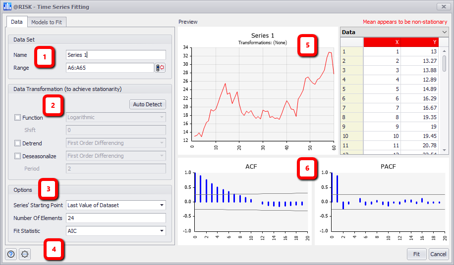
Figure 1 - Time Series Fitting Window
Time Series Fitting Window
The Data tab of the Time Series Fitting window contains the following primary sections:
- Data Set - Details of the data to be included in the Fit, including a Name value which appears as the heading to the graph as well as the value in the Name column of the Model Window.
Please note: It is recommended to limit the Data Set used in fitting to 100,000 data points.
It is possible to fit larger data sets. However, the fitting process may take significantly longer; how much longer depends on several factors including:
- The full size of the data set
- If the "Auto Detect" option is enabled in Batch Fitting
- The Time Series model in use (e.g. AR1 and AR2 are faster to fit than BMMRJD
- Data Transformations - Configure any transformations that should be applied to the data for the fitting process. See Fit Data Transformations for more information.
- Options - Configure options for the fitting process, including how many elements to create in the resulting time series function and the fit statistic to use for determining the best fit. See Fit Data Options for more information. Please note that these options can also be changed when viewing the results of the fit; see Fit Time Series Results for more information.
- Command Buttons - See below for more information.
- Graph and Information Panels - The graph and data points (x,y coordinates) for the time series data set used in the fit. To view the legend, use the dropdown menu in the upper right corner of the graph.
- Autocorrelation Graphs - The Autocorrelation Function (ACF) and Partial Autocorrelation Function (PACF) graphs for the data set used in the fit. These graphs help determine stationarity.
Time Series Fitting Command Buttons
The Time Series Fitting window Command Buttons include the following options:
-
 Help - Open help resources (online or local, based on @RISK settings); see Help Button for more information.
 -
 Settings/Actions - Window-specific settings and actions. The available options are: