Define Time Series Correlation
The Define Time Series Correlation command will cause two or more time series to no longer be completely independent of one another, but instead to be governed by a correlation matrix.
Much like correlations of @RISK distributions, time series correlations add the RiskCorrmat property function to the time series functions. For example, the following time series function:
{=RiskAR1(0,0.05,0.25,0)}
Is updated as follows when added to a correlation matrix named "MyCorrelation":
{=RiskAR1(0,0.05,0.25,0,RiskCorrmat(MyCorrelation,1))}
Specifying Inputs
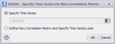
Figure 1 - Specify Time Series
When creating a new correlation matrix for a time series, the first window that opens is the Specify Time Series window which includes two options:
Once inputs have been specified, the Define Correlation window will open. See Define Correlation Window for more information.
Understanding Time-Series Correlation
It’s important to understand that correlations between time-series are fundamentally different from those between standard distributions. A correlation between two time series functions indicates that each iteration the array of values returned by the two time series are subject to the specified correlation coefficient. In contrast, the correlation between two standard @RISK distribution functions requires the entire simulation for that correlation to be apparent.
To understand how @RISK’s correlation is implemented, it is important to realize that time series models generate the value at a particular time based on one or more known values from previous time periods plus a randomly distributed noise term. It is the distributions of noise that obey the correlations you specify.
Also be aware that the correlations specified always apply to the underlying stationary time series model before any transformations (such as exponentiation or integration) are applied. A common way to generate correlated time series is by using the batch fit command, which as part of its output constructs a correlation matrix. The coefficients in that matrix will be the correlations between the data after all the specified data transformations have been applied to each of the series. For example, imagine there are two series of data that are stock prices. It is very common to use a log transform and first differencing to convert the raw values into period returns before fitting them. It is these returns, and not the raw series of data, for which the correlation coefficients are calculated.
Some time series functions, the so-called regressive models, have a state of equilibrium to which the series is strongly pulled if appreciable deviations from that equilibrium occur. If two time series are correlated, one or both of which are out-of-equilibrium at the start of the series, any correlation specified between them can be overwhelmed at the start of the forecast by the need for the series to bring itself back to the equilibrium state. Often the desired correlations are only actually realized after a “burn in” period where the series have settled back to equilibrium. (Incidentally, this also means that correlations for the BMMRJD time-series will only be approximate, since every time a jump occurs, its need to recover from that jump will overwhelm the effect of the correlations.)