Time Series Transformations

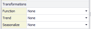
Figure 1 - Time Series Transformations

The Transformations section (Figure 1, right) of the Define Time Series window allows for the application of a number of transformations to the data for a time series. When both defining a time series and fitting a time series, transformations are primarily applied to achieve the level of stationarity as needed by the time series model that is being utilized. In the case of defining a time series model, generally transformations are applied to create non-stationary models (using Trend and Seasonalize), whereas with fitting transformations are used to achieve stationarity, which is required by the fitting process.

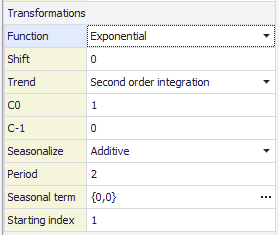
Figure 2 - Transformation, All Options

The options available in the Transformation panel will change based on the selections made for the three primary configurations. The full set of options (Figure 2, right) is discussed below.

Transformation Options

The three primary transformation configurations are Function, Trend, and Seasonalize. Selecting an option for any of the three configurations will update the Transformations panel with new options based on the selection made. The full options, with the associated choices are:

  • Function - Select to apply a transformation to the resulting time series model.
    • Exponential - Apply an exponential transformation to each value of the time series; exponential transformation is automatically applied when the selected model is GBM or GBMJD.
    • Square - Apply a square transformation to each value of the time series.
  • Shift - Only available when a Function (above) is selected. Apply a shift (e.g. add or subtract the configured value) to the time series data after the selected transformation (above) has been applied.
  • Trend - Define systematic change in the mean of time series values in terms of direction (increase or decrease).
    • First Order Integration - Add trend to the time series using a single integration; first order integration is automatically applied when the selected model is GBM or GBMJD.
    • Second Order Integration - Add trend to the time series using two integrations.
  • C0 - Only available when Trend (above) is set to 'First Order Integration' or 'Second Order Integration'. First starting constant - required to apply first order integration.
  • C-1 - Only available when Trend (above) is set to 'Second Order Integration'. Second starting constant - required to apply second order integration.
  • Seasonalize - Apply seasonality, or repetitive and predictable movement around the trend line.
    • First order integration - Add seasonality to the time series, applying one seasonal integration.
    • Second order integration - Add seasonality to the time series, applying two seasonal integrations.
    • Additive - Add seasonality to the time series where the amplitude of the seasonal effect is the same each season.
  • Period - Only available when Seasonalize (above) is set to a value other than 'None'. The number of data points in one seasonal period, e.g. '4' for a quarterly time series, '12' for monthly data, or '24' for hourly data.
  • Seasonal term - Only available when Seasonalize (above) is set to a value other than 'None'. Define the seasonal index; a seasonal index is the measure of how a particular point of one seasonal period changes compared to the average of that season. For first and second order integrations, this value is the integration constant. For additive seasonality this value represents the additive terms.
  • Starting index - Only available when Seasonalize (above) is set to 'Additive'. The starting index for the seasonal period when using additive seasonality; for example, this value would be '5' if using a monthly time series and the series begins in May instead of January.

There are two scenarios where transformations are automatically applied:

  1. If the selected time series model is GBM.
  2. After fitting a time series model to data that has been transformed.