Fit Data Transformations

Figure 1 - Topic Text
The fitting process for time series data requires stationarity. In a strict sense this means that the joint distribution of a time series can not vary over time. However, a more common, but weaker, definition of stationarity is that the statistics for the data (e.g. mean, standard deviation, etc.) are constant over time. For fitting many time series, such as ARMA, both definitions are equivalent.
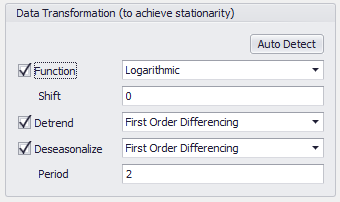
If the data are not naturally stationary, various transformations can be applied to achieve stationarity; these options are found in the Data Transformations section (Figure 1, right) of the Time Series Fitting and Time Series Batch Fitting windows.
Please note: the Auto Detect feature for determining Transformations uses a set of heuristics to determine "good guesses" for the transformations to apply to data. Though it is an educated guess, it is still a guess, and any transformation applied by Auto Detect should be checked for applicability!
If the time series data being used in the fitting process is already stationary, or if the details of the data are known, transformations can be applied manually. Otherwise, the 'Auto Detect' functionality can be used to have @RISK automatically evaluate transformations of the data that produce stationarity. @RISK uses a set of heuristics to determine likely transformations to apply to the data set before fitting.
For a single time series fitting, click the 'Auto Detect' button to apply the recommended transformations; these can always be modified before running the fit.
For a batch time series fitting, check the 'Auto Detect' checkbox to automatically apply the recommended transformations; unlike a single time series fit, the transformations cannot be modified before running the fit.
Fit Transformation Options
The three primary transformation configurations are Function, Detrend, and Deseasonalize; checking the box next to an option will enable it. Activating the Function option will enable adding a Shift, and activating Deseasonalize will enable adding a Period. The full options, with the associated choices are: