A Digital Example
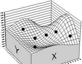
Figure 1 - Solution Landscape Possible Solutions
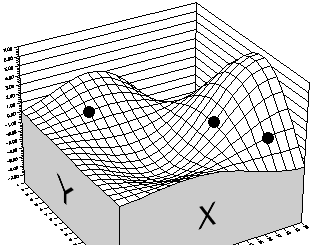
Figure 2 - Initial "Good" Solutions
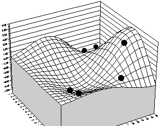
Figure 3 - Crossover Solutions
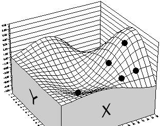
Figure 4 - New "Good" Solutions
Now consider a problem with two variables, X and Y, that produce a result Z. If the resulting Z for every possible X and Y values were calculated and plotted, a solution “landscape” would emerge. When trying to find the maximum “Z”, the peaks of the function are “good” solutions, and the valleys are “bad” ones.
When a genetic algorithm is used to maximize the function, it starts by creating several possible solutions or scenarios at random (the black dots), rather than just one starting point. It then calculates the function’s output for each scenario and plots each scenario as one dot. Next it ranks all of the scenarios by height, from best to worst. It keeps the scenarios from the top half and discards the others.
Each of the three remaining scenarios duplicates itself, bringing the number of scenarios back up to six. Now comes the interesting part: Each of the six scenarios is composed of two adjustable values, X and Y. The scenarios pair off with each other at random. Each scenario exchanges the first of its two adjustable values with the corresponding value from its partner.
For example:
| Before | After | |
| Scenario 1 | 3.4, 5.0 | 2.6, 5.0 |
| Scenario 2 | 2.6, 3.2 | 3.4, 3.2 |
This operation is called crossover. When the six scenarios randomly mate and perform crossover, there is a new set of scenarios:
In the above example, the original three scenarios, a, b, and c, paired up with the duplicates, A, B, C, to form the pairs aB, bC, bA. These pairs then switched values for the first adjustable cell, which is equivalent in the diagram to exchanging the x and y coordinates between pairs of dots. The population of scenarios has just lived through a generation, with its cycle of “death” and “birth.”
Notice that some of the new scenarios result in lower height than any in the original generation. However, one scenario has moved high up on the tallest hill, indicating progress. If the population evolves for another generation, it might lead to the scenario in Figure 4, right.
It should be clear how the average performance of the population of scenarios increases over the last generation. In this example, there is not much room left for improvement. This is because there are only two genes per organism, only six organisms, and no way for new genes to be created - there is a limited gene pool. The gene pool is the collection of all the genes of all organisms in the population.
Genetic algorithms can be made much more powerful by replicating more of the inherent strength of evolution in the biological world; increasing the number of genes per organism, increasing the number of organisms in a population, and allowing for occasional random mutations. In addition, the algorithms can choose the scenarios that will live and reproduce with a random element that has a slight bias towards those that perform better, instead of simply choosing the best performers to breed.