RiskBinomial

Description

RiskBinomial(n, p) specifies a binomial distribution with parameters n and p. This is usually used to model the number of “successes” in n independent, identical trials, where p is the probability of success on each trial.

For example, RiskBinomial(10,20%) represents the number of discoveries of oil from a portfolio of 10 prospects, where each prospect has a 20% chance of having oil. An important modelling application is when n=1, so that there are two possible outcomes (0 or 1), where the 1 has probability p, and the 0 has probability 1-p. (In this case, it is equivalent to the RiskBernoulli function with parameter p.) With p=0.5, it is equivalent to tossing a fair coin. For other values of p, the distribution can be used to model event risk, that is, the occurrence or nonoccurrence event, or to transform registers of risks into simulation models to aggregate the risks.

Examples

RiskBinomial(5,0.25) returns a binomial distribution generated from 5 trials with a 25% probability of success on each trial.

RiskBinomial(C10*3,B10) returns a binomial distribution generated from the number of trials taken from the value in cell C10 times 3. The probability of success on each trial is taken from cell B10.

Guidelines

n must be a positive integer less than or equal to 32,767.

p must be between 0 and 1.

Parameters

n discrete “count” parameter n > 0 *

p continuous “success” probability 0 < p < 1 *

*n = 0, p = 0 and p = 1 are supported but give degenerate distributions.

Domain

discrete integers

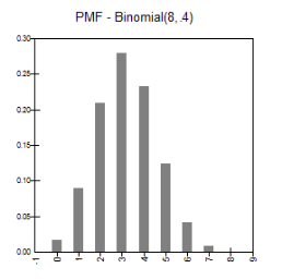
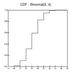
Mass and Cumulative Distribution Functions

Mean

Variance

Skewness

Kurtosis

Mode

(bimodal)       and
if is integral

(unimodal)      largest integer less than otherwise

Examples