Sampling Methods
Sampling is the process by which values are randomly “drawn” from input probability distributions. For each distribution, one sample value is created for each iteration performed.
Statisticians and practitioners have developed several techniques for drawing random samples. The two methods of sampling used in @RISK, Monte Carlo sampling and Latin Hypercube sampling, differ in the number of iterations required until sampled values approximate input distributions to any degree of accuracy. Monte Carlo sampling often requires a larger number of samples, especially if the input distribution is highly skewed or has some outcomes of low probability. Latin Hypercube sampling forces the samples drawn to correspond more closely with the input distribution, and it converges faster.
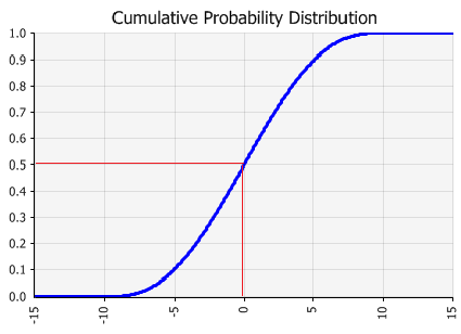
Figure 1 - Cumulative Probability Example
For this discussion, it’s helpful to first understand the concept of a cumulative distribution. Any probability distribution may be expressed in cumulative form. A cumulative curve (Figure 1, right) is scaled from 0 to 1 on the Y-axis, with Y-axis values representing the cumulative probability up to the corresponding X-axis value.
In the cumulative curve illustrated in Figure 1, the 0.5 cumulative value is the point of 50% cumulative probability (0.5 = 50%). Fifty percent of the values in the distribution fall below this median value and 50% are above. The 0 cumulative value is the minimum value (0% of the values will fall below this point) and the 1.0 cumulative value is the maximum value (100% of the values will fall below this point).
Why is this cumulative curve so important to understanding sampling? The 0 to 1 scale of the cumulative curve is the range of the possible random numbers generated during sampling. In a typical sampling sequence, the computer will generate a random number between 0 and 1, with any number in the range equally likely to occur. This number is then used to select a value from the cumulative curve. In the example graph, the value sampled for the distribution shown would be X1 if a random number of 0.5 was generated during sampling. Because the shape of the cumulative curve is based on the shape of the input probability distribution, it is more probable that more likely outcomes will be sampled. The more likely outcomes are in the range where the cumulative curve is the steepest.
Monte Carlo Sampling
Monte Carlo sampling refers to the traditional technique for generating random or pseudo-random numbers to sample from a probability distribution. The term Monte Carlo was introduced during World War II, as a code name for the simulation of problems associated with the development of the atomic bomb. Today, Monte Carlo techniques are applied to a wide variety of complex problems involving random behavior. A wide variety of algorithms are available for generating random samples from different types of probability distributions.
Actually, the term Monte Carlo is used in two ways in @RISK. It is used to describe the overall simulation process, as in ”Monte Carlo simulation.” This distinguishes @RISK-type simulations from other types of simulation, such as discrete-event simulations. However, the second use of the term, “Monte Carlo sampling,” is more restrictive and is relevant to the current discussion. This term applies only to the way random values are generated during a simulation. Another way to say it is that you can perform either Monte Carlo sampling or Latin Hypercube sampling in a Monte Carlo simulation.

Figure 2 - Monte Carlo Sampling Example
When Monte Carlo sampling is performed, each draw from a uniform distribution over 0 to 1 is independent of each other draw, with one draw per iteration for each input distribution. Each of these draws provides a Y value for the cumulative curve, which is then mapped to the relevant X value as shown in the above graph. This is a perfectly acceptable procedure in the “long run,” but in the “short run” (a small number of draws), it can lead to clustering, where not all of the relevant distribution is represented.
Figure 2, right, illustrates this clustering. The five generated Y values just happen to be close to each other. This leads to five X values close to one another as well. The rest of the X values haven’t been sampled at all.
Clustering becomes especially pronounced when a distribution includes low probability outcomes, which could have a major impact on your results. It is important to include the effects of these low probability outcomes. To do this, these outcomes must be sampled, but if their probability is low enough, a small number of Monte Carlo iterations might not sample sufficient quantities of these outcomes for inclusion in your simulation model. This problem has led to the development of stratified sampling techniques such as the Latin Hypercube sampling used in @RISK.
Latin Hypercube Sampling
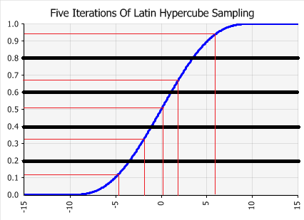
Figure 3 - Latin Hypercube Sampling Example
Latin Hypercube sampling is a more recent development in sampling technology. It is designed to avoid the clustering that can occur with Monte Carlo sampling. The key to Latin Hypercube sampling is the stratification of the input probability distributions. Stratification divides the cumulative curve into equal intervals on the cumulative probability scale (0 to 1). A sample is then randomly taken from each interval or “stratification” of the input distribution. Sampling is forced to represent values in each interval. Therefore, all values in the input distribution have a better chance at being sampled.
In the following graph, the Y axis has been divided into five intervals. During sampling, for every five draws, one of the draws will fall in each of the five intervals; they can’t cluster as in the Monte Carlo method. With Latin Hypercube, the samples are guaranteed to more accurately reflect the distribution of values in the input probability distribution.
When not to Use Latin-Hypercube
In general Latin-Hypercube is the superior sampling method. It converges more quickly to a stable set of results than the Monte-Carlo sampling method. However, if you are trying to reproduce standard statistical result (e.g. an empirical confirmation of the central limit theorem) the Monte-Carlo method will be required.