RiskNormal
|
Description |
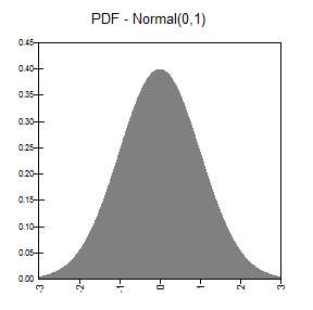
RiskNormal(mean,standard deviation) specifies a normal distribution with parameters mean and standard deviation. This is the traditional “bell shaped” curve. The use of the normal distribution can often be justified by a mathematical result called the Central Limit Theorem. This states essentially that the sum of many random quantities is approximately normally distributed, regardless of the distributions of the quantities in the sum. Therefore, the normal distribution can be used to represent the uncertainty of a model’s input whenever the input is the result of many random processes acting together in an additive manner. Examples could include the total number of goals scored in a soccer season or the amount of oil in the world (assuming that there are many reservoirs of approximately equal size, each with an uncertain amount of oil). Two potential drawbacks of the normal distribution for real applications are (1) it is symmetric, not skewed, and (2) it allows negative values. However, if the mean is positive and is at least 3 or 4 times larger than the standard deviation, the probability of a negative value is fairly negligible. (In any case, the RiskTruncate property function can be used to ensure that no negative values are sampled.)
|
|
Examples |
RiskNormal(10,2) returns a normal distribution with mean 10 and standard 2. RiskNormal(SQRT(C101),B10) returns a normal distribution with mean equal to the square root of the value in cell C101 and standard deviation taken from cell B10.
|
|
Guidelines |
standard deviation must be positive. |
|
Parameters |
*σ = 0 is supported but gives a degenerate distribution with x = μ. |
|
Domain |
|
|
Density and Cumulative Distribution Functions |
Here, Φ is called the cumulative distribution for N(0,1), and erf is the error function.
|
|
Mean |
|
|
Variance |
|
|
Skewness |
0
|
|
Kurtosis |
3
|
|
Mode |
|
|
Examples |
|
 continuous location parameter
 continuous scale parameter
 continuous